Reading a SQL Execution Plan: EXPLAIN and EXPLAIN ANALYZE Without the Jargon
What your database is actually doing when it runs a query — scan types, join algorithms, cost estimates, and the specific signs that tell you where a slow query is actually losing time.
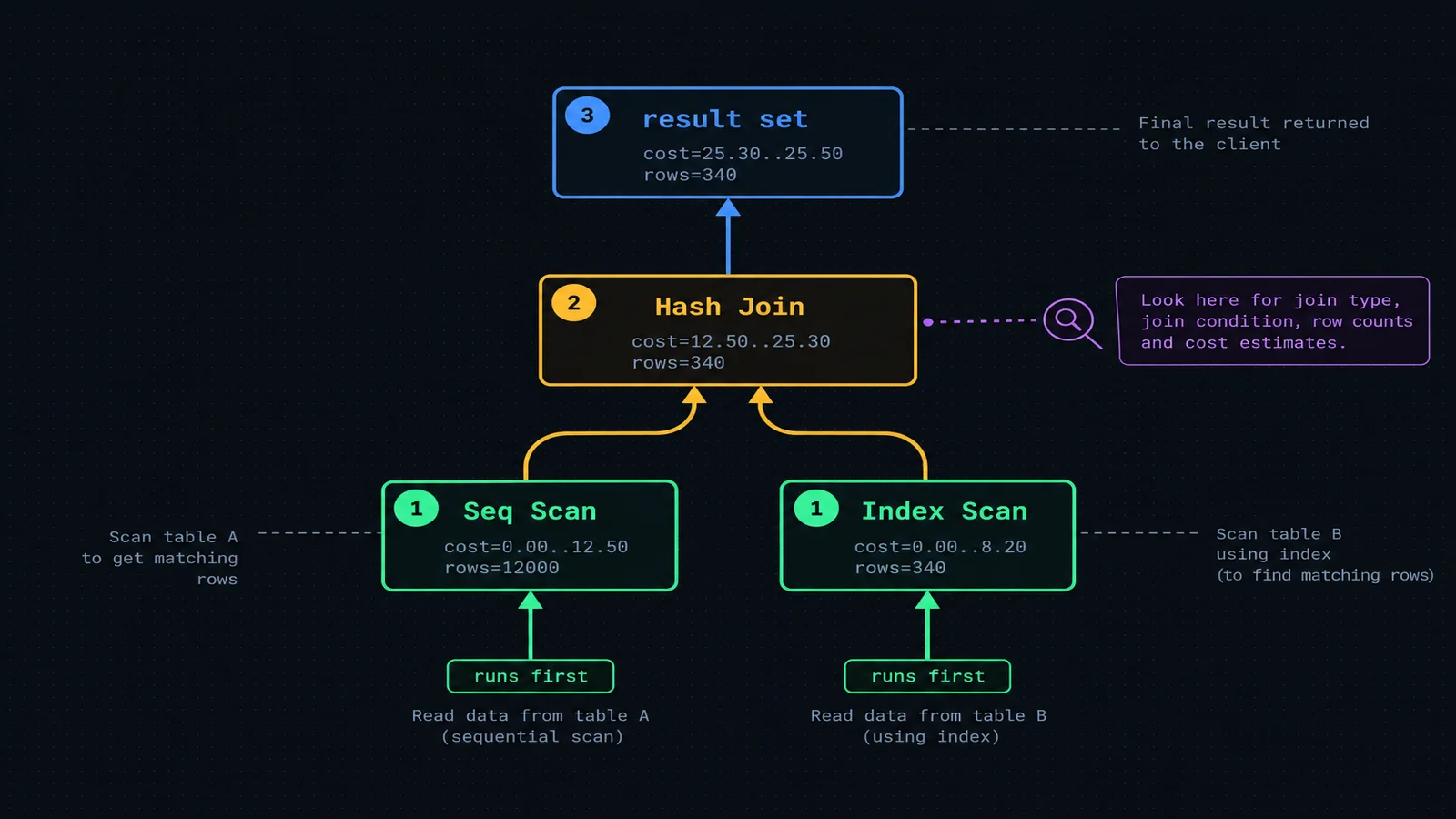
Ask most SQL developers what happens after they hit run and the honest answer is "the database figures it out." That's true, and it's also the reason so many performance problems get fixed by luck instead of by diagnosis — someone adds an index, or rewrites a join, or throws a LIMIT on the end, and the query gets faster, and nobody can tell you exactly why, which means nobody can tell you whether the next slow query needs the same fix or a completely different one. An execution plan closes that gap. It's the one artifact that tells you, in specific and falsifiable terms, what the engine actually did — not what the SQL implies it should do, not what worked last time, but the literal sequence of scans, joins, sorts, and filters that produced your result set, along with how much each step cost.
This article is a field guide to reading that artifact across the four engines most data people actually touch day to day: Postgres, MySQL, Snowflake, and BigQuery. The syntax differs, the UI differs, but the underlying concepts — scan types, join algorithms, cost estimation, the gap between what the optimizer expected and what actually happened — are close to universal, because they all describe the same handful of physical operations a relational engine can perform on a table. Learn to read one plan well and the other three become a vocabulary problem, not a conceptual one.
Why Look at a Plan At All
SQL is declarative. You write WHERE order_status = 'shipped' and the database decides how to find those rows — scan the whole table and check every row, walk an index and jump straight to the matches, or something else entirely depending on what indexes exist, how selective the filter is, and how large the table has grown since anyone last checked. Two queries that are byte-for-byte identical in their SQL text can execute completely differently on the same table six months apart, purely because the data distribution changed and the optimizer's decision changed with it. The SQL text describes the destination. The execution plan describes the route, and the route is the only thing that actually costs time.
That distinction matters because most performance intuition is built on the SQL text, not the route. It's natural to look at a query with five joins and assume the joins are the expensive part, or to see a subquery and assume subqueries are inherently slow, or to see a missing LIMIT and assume that's the bottleneck. Sometimes one of those guesses is right. Often it isn't, and the actual cost is concentrated somewhere unglamorous — a single filter on a non-indexed column forcing a full scan of a table three other joins depend on, for instance — that no amount of staring at the SQL text alone would reveal. We covered this same principle from the query-authoring side in our piece on SQL and dbt query optimization: optimize the step the plan says is expensive, not the step that looks the most complicated in the SQL. This article is the other half of that advice — it's about actually being able to read the plan in the first place, node by node, engine by engine, well enough to know which step that is.
There's a second, quieter reason to build this skill even when nothing is currently slow. A plan tells you not just what happened, but what the optimizer believed about your data going in — how many rows it expected a filter to return, how selective it thought a join predicate was. When that belief is wrong, the plan is often still "correct" in the sense that it executes without error and returns the right rows, but it's the wrong plan for the data that actually exists, chosen based on a stale or inaccurate estimate. Catching that gap early, before it turns into a production incident, is one of the most useful habits a data engineer can build, and it's impossible without knowing how to read what the plan is telling you on both sides of that estimate. If you want to practice on a real query without setting up a database first, tools.techedge.in's SQL explainer is a reasonable place to paste a plan and see it annotated node by node while you're still building the muscle memory this article is trying to teach.
EXPLAIN vs. EXPLAIN ANALYZE
Every major engine gives you two distinct ways to ask "what will you do with this query," and conflating them is the single most common mistake people make when they're new to reading plans. EXPLAIN alone asks the optimizer to show you its intended plan without running the query — it's a prediction, built entirely from statistics the engine has already collected about your tables (row counts, distinct value estimates, histograms of value distribution) and the cost model it uses to compare candidate plans against each other. Nothing gets executed. No rows come back. You get the plan, and only the plan, in milliseconds, regardless of how long the query itself would actually take.
EXPLAIN ANALYZE is a different thing entirely: it actually executes the query, start to finish, and then reports the same plan shape annotated with what really happened at each step — real elapsed time, real row counts, real number of times each step ran. This is the crucial distinction to internalize before you run it against anything that isn't a plain read: EXPLAIN ANALYZE runs the query for real. On a SELECT, that's harmless beyond the time and resources the query itself consumes. On an UPDATE, DELETE, or INSERT, it actually performs the write — Postgres's own documentation is explicit that EXPLAIN ANALYZE on a data-modifying statement will execute it, so the standard safe pattern is to wrap it in a transaction and roll back afterward rather than run it bare against production data.
EXPLAIN
SELECT order_id, order_status, order_total
FROM orders
WHERE order_status = 'shipped'
AND order_date >= current_date - INTERVAL '7 days';EXPLAIN (ANALYZE, BUFFERS)
SELECT order_id, order_status, order_total
FROM orders
WHERE order_status = 'shipped'
AND order_date >= current_date - INTERVAL '7 days';The BUFFERS option, only meaningful alongside ANALYZE, adds a further layer of truth: how many pages were served from Postgres's shared buffer cache (shared hit) versus how many had to be pulled from disk or the OS page cache (shared read). A plan that looks fast on a warm cache and slow on a cold one is an extremely common source of "it was fast when I tested it and slow in production" confusion, and BUFFERS is usually the fastest way to confirm that's what's happening rather than guess at it.
The practical rule of thumb: reach for plain EXPLAIN when you want to sanity-check what the optimizer intends to do before running something expensive or destructive — a good habit before running a heavy backfill, for instance — and reach for EXPLAIN ANALYZE (with BUFFERS on Postgres specifically) when a query is already slow and you need to know where the actual time went, not the predicted time. The estimated plan alone can mislead you in exactly the cases you care about most, because a stale statistics table produces a confidently wrong estimate that only ANALYZE's real execution numbers will expose — which is precisely the subject of the red flags section further down.
Reading the Tree: Nodes, Indentation, and Execution Order
An execution plan is a tree, and the single fact that unlocks reading one correctly is this: the innermost, most-indented nodes execute first. Data flows upward and outward from the bottom of the tree to the top — the deepest, most nested operation runs, produces some rows, and hands them to the node directly above it, which does something with those rows (filters them, joins them to another input, sorts them) and hands its own output further up, until the topmost node produces the final result set that gets returned to you. This is the opposite of how most people instinctively read the SQL that generated the plan, where SELECT appears first and WHERE appears further down — the plan's execution order has almost nothing to do with the order clauses appear in the query text.
Hash Join  (cost=45.32..892.14 rows=1200 width=64)
  Hash Cond: (o.customer_id = c.customer_id)
  -> Seq Scan on orders o  (cost=0.00..812.00 rows=8400 width=48)
       Filter: (order_status = 'shipped'::text)
  -> Hash  (cost=32.10..32.10 rows=1058 width=24)
       -> Seq Scan on customers c  (cost=0.00..32.10 rows=1058 width=24)
Read this bottom-up. The two Seq Scan nodes are the deepest, most-indented operations — they run first, each independently reading its own table. The scan on customers feeds into a Hash node, which builds an in-memory lookup structure from those rows. Only once both inputs are ready does the top-level Hash Join node run, probing the hash table with each row streaming out of the orders scan. Nothing about that sequence is visible from reading the original SQL top to bottom — you'd have to already know how a hash join works to guess it, which is exactly why the plan, not the query text, is the thing worth learning to read directly.
MySQL's tree-format output (the format EXPLAIN ANALYZE always uses, from MySQL 8.0.18 onward) makes this same bottom-up structure even more explicit, using nested -> arrows and indentation to represent the same iterator-based execution model — each line is literally an iterator that pulls rows from the iterator nested one level deeper than it. Snowflake's Query Profile and BigQuery's execution graph both render this as an actual visual tree or DAG rather than indented text, but the underlying rule doesn't change: leaf nodes at the bottom or edges of the graph are where data enters the plan, and everything flows toward a single root or final stage that represents your result set.
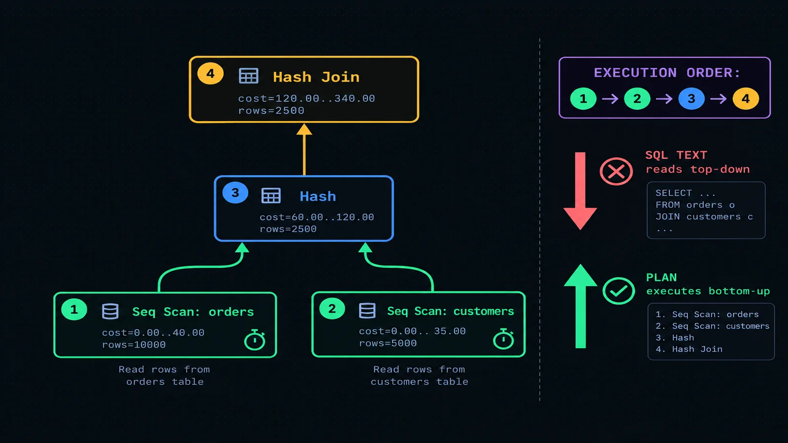
One more habit worth building early: read a plan for shape before you read it for numbers. Before worrying about any specific cost or row count, just trace which nodes are leaves, which nodes combine two inputs (joins), and which nodes transform a single input (filters, sorts, aggregates). That shape alone — three scans feeding two joins feeding a sort, say — already tells you the rough structure of the work being done, and it's much easier to spot an obviously wrong shape (a full scan where you expected an index lookup, an extra sort you didn't ask for) than it is to spot a subtly wrong number on first read.
Scan Types: Seq Scan, Index Scan, Index-Only Scan, Bitmap Scan
Every plan bottoms out at leaf nodes that read data from a table, and which specific scan type appears at each leaf is usually the single biggest lever on that node's cost. There are four scan types worth knowing cold, and they trade off against each other based almost entirely on selectivity — what fraction of the table actually matches your filter.
Seq Scan (sequential / full table scan)
A sequential scan reads every page of a table, in physical storage order, checking each row against any filter conditions as it goes. It sounds naive, and for a highly selective filter on a huge table it usually is the wrong choice — but for a large fraction of the table, or for a genuinely small table, it's frequently the correct choice, because the overhead of jumping around an index and then fetching each matching row individually from scattered locations on disk can exceed the cost of just reading the whole table in one efficient, sequential pass. A seq scan showing up in a plan is not automatically a problem; a seq scan on a filter that should only match 0.1% of a 40-million-row table is.
Index Scan
An index scan walks a B-tree (or equivalent) index structure to find matching entries, then, for each match, jumps to the corresponding row in the table's heap storage to fetch the actual column values not present in the index itself. This is efficient specifically because the index lets the engine avoid reading rows that can't possibly match — but each heap fetch is a separate, potentially random-access read, so an index scan that matches a large fraction of the table can actually cost more than a seq scan would have, which is exactly why the optimizer weighs selectivity, not just "does an index exist," when choosing between the two.
Index-Only Scan
When every column a query needs is present in the index itself, the engine can skip the heap fetch entirely and answer straight from the index — an index-only scan. This is the fastest of the four when it's available, which is why "covering indexes" (indexes that include every column a hot query touches, not just the filter column) are a deliberate design technique, not an accident. The catch worth knowing: Postgres can only skip the heap fetch for a given page if that page is marked "all-visible" in the visibility map, meaning no recent updates or deletes need row-visibility rechecking. A table with a lot of recent write activity and infrequent vacuuming can show an index-only scan that still reports a nonzero Heap Fetches count in EXPLAIN ANALYZE output — a sign the index-only scan isn't actually getting its full benefit, and that the table could use a vacuum before you conclude the covering index itself is the problem.
Bitmap Scan (Bitmap Index Scan + Bitmap Heap Scan)
A bitmap scan is Postgres's answer to the middle ground between "too many matches for an index scan to be efficient" and "too few matches to justify a full seq scan." It happens in two steps, shown as two separate plan nodes: a Bitmap Index Scan walks the index and builds an in-memory bitmap marking which heap pages contain at least one matching row, then a Bitmap Heap Scan reads only those flagged pages, in physical page order rather than index order — turning what would otherwise be scattered random-access reads into a smaller number of sequential reads. It's also the mechanism Postgres uses to combine two separate indexes on the same table for a single query (via BitmapAnd or BitmapOr nodes), something a plain index scan can't do on its own since it can only walk one index at a time.
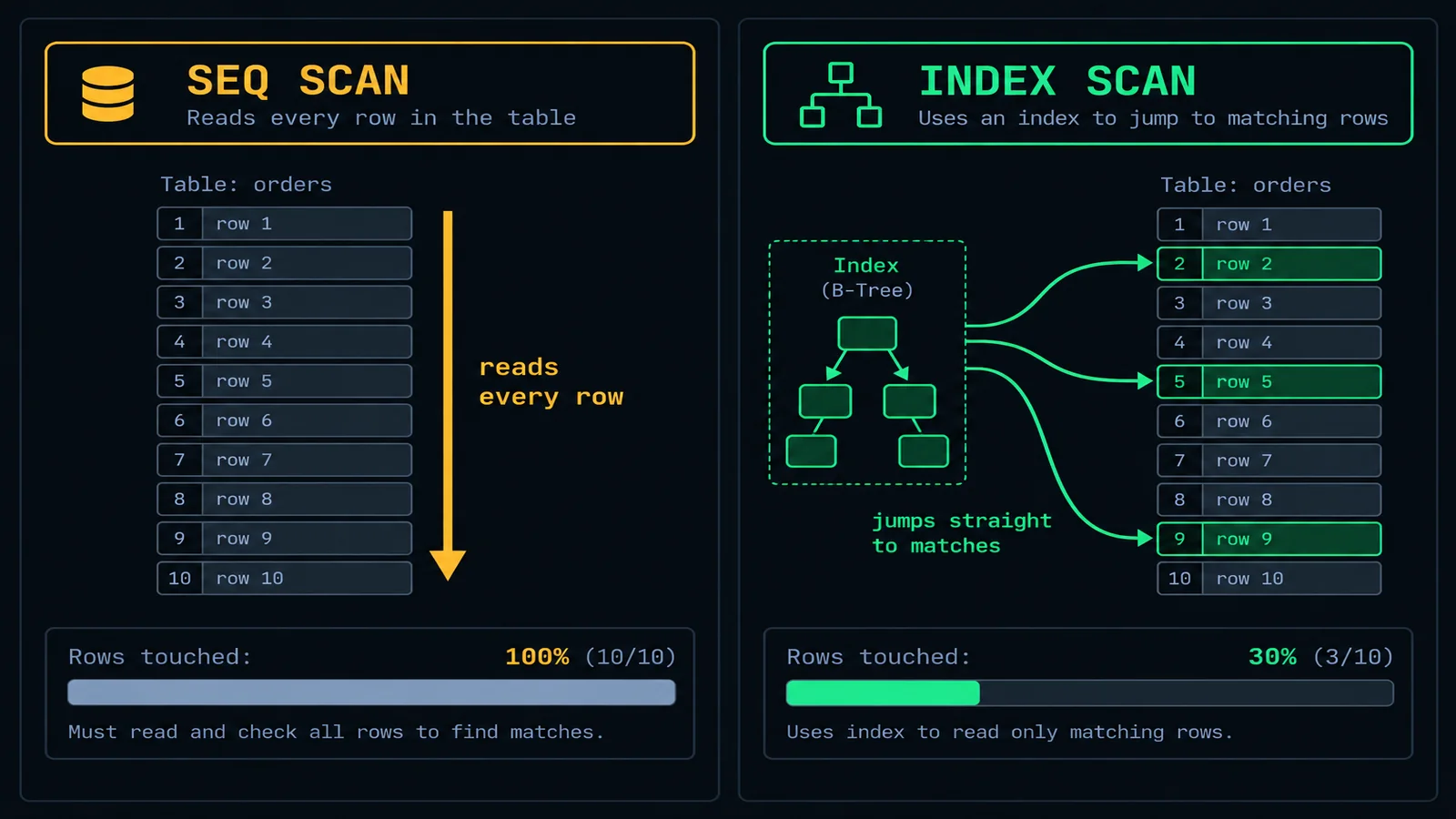
MySQL's terminology maps closely but not identically: its EXPLAIN output reports an access type column per table (values like ALL for a full scan, index for a full index scan, range, ref, or eq_ref for progressively more selective index lookups, and const for the fastest case of a single-row primary-key or unique-key lookup) rather than separate named node types the way Postgres does — but the underlying spectrum from "read everything" to "jump straight to the match" is the same idea wearing different labels. The general lesson generalizes across every engine in this article: the more selective your filter and the better it lines up with an available index (or, on Snowflake and BigQuery, with how the table is physically clustered and partitioned), the less data the leaf node has to touch to do its job.
Join Algorithms in the Plan: Nested Loop, Hash Join, Merge Join
Once a plan has more than one leaf node, something has to combine their outputs, and that's where join algorithms come in. Every mainstream relational engine picks between the same three physical join strategies, and which one gets chosen for a given join is one of the most informative signals in the entire plan — the optimizer is effectively telling you, through its choice, what it believes about the size and shape of the data on each side of the join. Our deep dive on SQL joins covers join semantics — what an inner join versus a left join actually returns — this section is about the physical mechanics underneath any of those, regardless of which logical join type you wrote.
Nested Loop
The conceptually simplest strategy: for every row produced by the outer (first) input, scan the inner (second) input looking for matches. Written naively that's O(n × m) and disastrous on two large tables — but it's frequently the best choice when the outer side is small (a handful of rows after filtering) and the inner side has a usable index on the join column, because then each of those few outer rows triggers one cheap indexed lookup rather than a full scan of the inner table. A nested loop is the plan you want when one side of a join is tiny; it's the plan that quietly destroys performance when the optimizer mistakenly believes one side is tiny and it actually isn't.
Hash Join
The workhorse for joining two larger inputs on an equality condition. The engine builds an in-memory hash table from the smaller of the two inputs (the "build" side), keyed on the join column, then streams the larger input (the "probe" side) through it, looking up each row's join key in the hash table in roughly constant time. No index is required on either side for a hash join to work well, which is why it's so often the optimizer's fallback when neither input has a convenient index — it turns an unindexed equality join into something close to linear-time work instead of the quadratic cost a nested loop would incur on the same inputs. The cost that hash joins can hit: the hash table has to fit comfortably in the memory budget the engine allots for the operation (Postgres's work_mem, for example); when it doesn't, the join spills to disk in batches, which is measurably slower and one of the concrete red flags covered next.
Merge Join
Requires both inputs to already be sorted on the join key — or willing to pay the cost of sorting them first. Given two sorted streams, a merge join walks both simultaneously in a single linear pass, advancing whichever pointer is currently behind, which makes it extremely efficient when the sort is "free" because the data already arrives in that order — from an index that's naturally ordered by the join column, or from a table clustered on it. It's also well suited to range-based join conditions (ON a.start_date <= b.event_date) where a hash join's pure-equality lookup doesn't apply at all. When the inputs aren't already sorted, the optimizer has to weigh the upfront sort cost against a hash join's build cost, and which one wins is entirely a function of input size and existing order — there's no universal answer, which is exactly why this is the optimizer's decision to make, not something worth hard-coding an opinion about in advance.
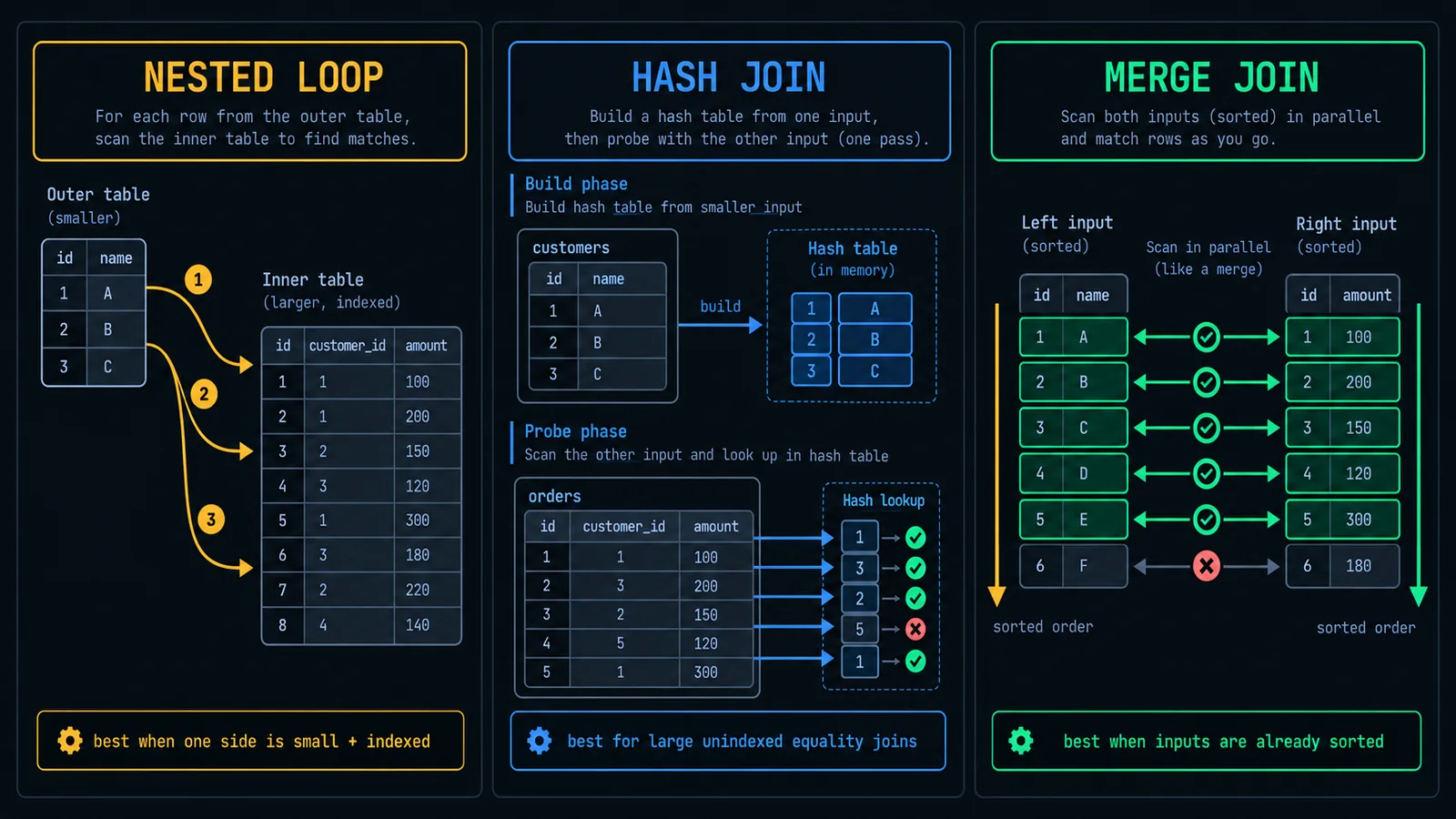
What decides which algorithm the optimizer picks, in practice, is almost always some combination of four things: the estimated size of each input after any filters are applied, whether a usable index exists on the join column for either side, whether the join condition is a plain equality or something else (a range, an inequality, a non-equality expression), and the memory budget available for building a hash table or performing a sort. Change any one of those — add an index, a filter gets more selective as the table grows, the memory setting changes — and the same logical join, written identically, can switch algorithms entirely on the next run. That's not a bug; it's the optimizer correctly responding to a changed situation. It's also exactly why a plan captured once, months ago, when someone was debugging a different problem, isn't a substitute for looking at the plan again today.
Cost, Rows, Width, and Actual Time: What the Numbers Actually Mean
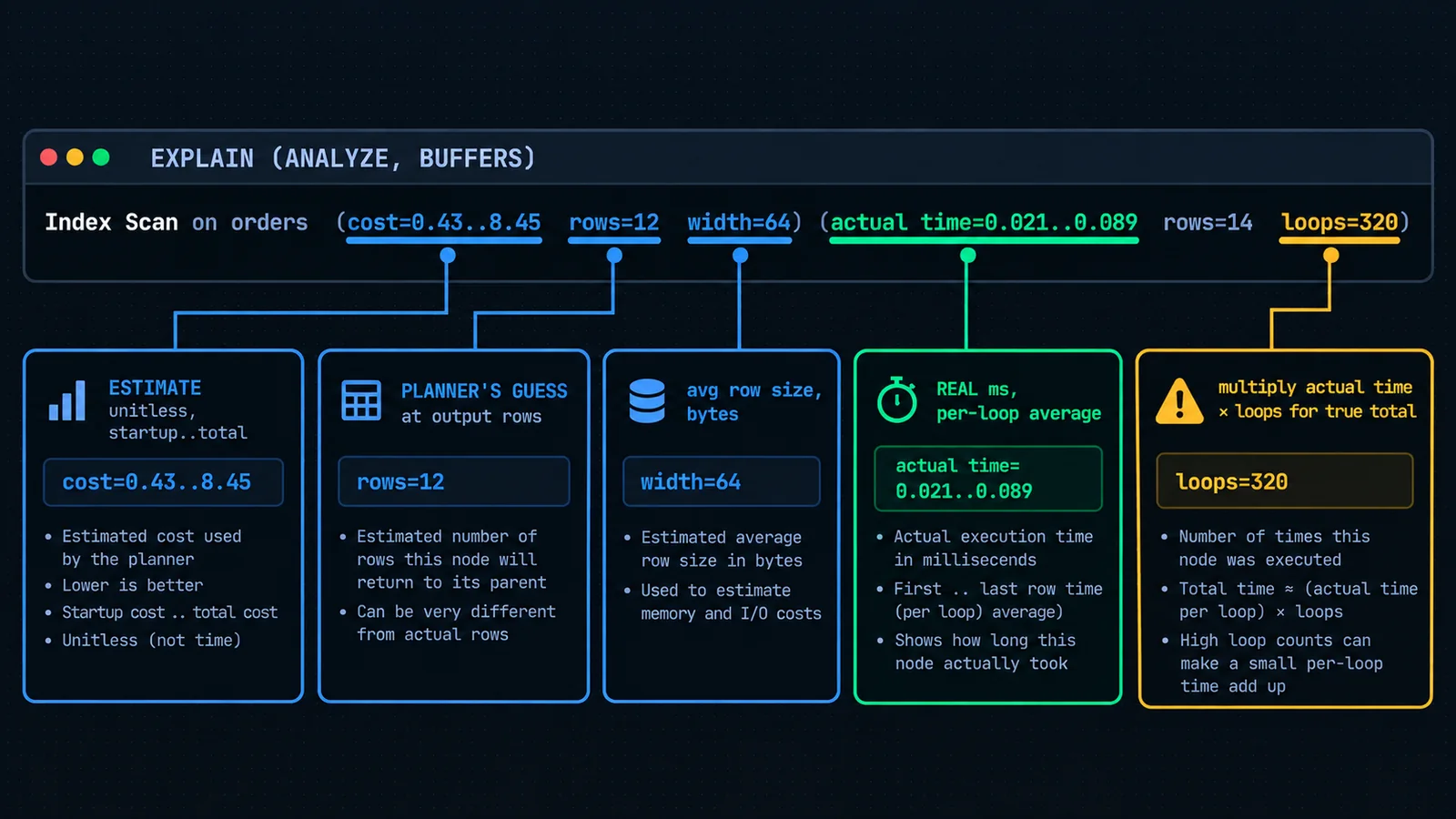
Every node in a Postgres or MySQL plan carries a cluster of numbers that looks intimidating until you know what each one is actually measuring. Take a single line from a real plan:
Index Scan using idx_orders_customer_id on orders  (cost=0.43..8.45 rows=12 width=64)
                                                    (actual time=0.021..0.089 rows=14 loops=320)
Cost is a pair of numbers — startup cost and total cost, separated by two dots — and both are unitless, relative figures, not milliseconds or any real-world time unit. They're computed by the planner from a cost model built out of tunable constants (Postgres's seq_page_cost, random_page_cost, cpu_tuple_cost, and a handful of others), combined with the planner's row-count estimates for that node. Startup cost is how much work happens before the node can produce its first row of output — for a plain index scan that's small, but for something like a sort, startup cost can be nearly as large as total cost, because a sort typically can't emit anything until it's processed its entire input. Total cost is the estimated cost of running the node to completion. The only thing cost numbers are good for is comparing candidate plans against each other — the optimizer picks whichever full plan has the lowest total cost at the root. They are not a time estimate, and treating a cost of "8.45" as "8.45 milliseconds" is a category error worth un-learning early.
Rows, in the estimated half of the line, is the planner's guess at how many rows this node will output after any filter condition at that node is applied — not how many rows it reads, but how many survive. It's derived from table statistics: row counts, most-common-value lists, histograms, and (where the engine supports it) cross-column correlation statistics. Width is the estimated average size, in bytes, of each output row, used partly for further cost calculations further up the tree and partly to help downstream operations like sorts and hash tables plan how much memory they'll need.
Actual time, which only appears with ANALYZE, is a startup..total pair exactly like cost, except measured in real milliseconds from the real execution — with one detail that trips people up constantly: it's the average time per loop, not the total time contributed by that node. The loops figure tells you how many times the node executed — a nested loop's inner side, for instance, runs once per row coming from the outer side, so its actual time reflects one execution and has to be multiplied by the loop count to get that node's real total contribution. A node reporting actual time=0.021..0.089 and loops=320 didn't cost 0.089ms total — it cost roughly 0.089 × 320 ≈ 28.5ms, and missing that multiplication is one of the most common ways people misjudge which node in a plan is actually the expensive one.
MySQL's EXPLAIN ANALYZE tree format reports the same conceptual pair per node — estimated cost and rows from the optimizer, alongside actual measured time and rows from the real execution, with its own loops figure for repeated sub-trees — so the reading discipline transfers directly even though the syntax looks different on the page. Snowflake and BigQuery don't expose an equivalent unitless cost number at all; instead they report real, already-executed statistics per operator or per stage — bytes scanned, rows produced, elapsed time, percentage of total query time — because their profiling tools only exist after a query has actually run, which is worth keeping in mind heading into the next section on how the four engines diverge.
Spotting Red Flags
Reading a plan node by node is a skill; knowing which nodes deserve your attention out of a plan with fifteen of them is a different, more practical skill, and it comes down to recognizing a short list of patterns that reliably indicate something is actually wrong, as opposed to merely present. None of these five require deep internals knowledge to spot once you know to look for them.
A seq scan on a table with a large row count, under a filter that should be highly selective. A seq scan by itself is not a problem — plenty of small tables and low-selectivity filters are correctly served by one. It becomes a red flag specifically when the table is large, the filter looks like it should match a small fraction of rows, and no index exists (or an index exists but isn't being used) to serve it more cheaply. Check the estimated rows against the table's total row count first; if the ratio is small and it's still choosing a full scan, that's the signal to look for a missing or unused index.
Estimated rows wildly different from actual rows. This is the single most diagnostic red flag in the entire plan, because it directly exposes a wrong belief the optimizer had going in — stale statistics, a correlated-column assumption the planner can't see, or a parameter value the planner had to guess at generically. A node estimated at 12 rows that actually returns 40,000 is a strong signal the optimizer picked a plan (often a nested loop, since those only make sense for small inputs) that's completely wrong for the data that's actually there, and no amount of rewriting the SQL will fix it until the underlying statistics problem is addressed.
An expensive sort consuming a large share of total time. Sorts are common, necessary, and frequently fine — but a sort operating over a huge unfiltered input, especially one feeding a merge join or an ORDER BY with no matching index, can dominate a plan's runtime disproportionately to how "important" that step looks in the SQL. Check whether the sort could be avoided entirely with an index that already provides the needed order, or whether the input to the sort could be filtered down first.
Disk spill on a sort or hash operation. In Postgres, a sort that doesn't fit in the memory budget (work_mem) reports Sort Method: external merge along with a Disk: figure in the plan output — a direct sign the engine had to write intermediate data to disk and merge it back, which is materially slower than an in-memory sort. A hash join facing the same memory pressure spills into multiple batches instead of one, visible as a Batches figure greater than one on the Hash node. Either one is a concrete, unambiguous signal, not a matter of interpretation — it's either spilling or it isn't, and the plan tells you directly.
A small per-loop actual time hiding a large total, because of the loops trap covered above. A node with actual time=0.02..0.09 looks trivially fast in isolation. The same node with loops=50,000 is not trivial at all — it's the largest single contributor to the query's total runtime, just distributed across many small executions instead of concentrated in one. This is the red flag most likely to be missed on a fast skim of a plan, precisely because each individual number looks unremarkable; it only shows up once you do the multiplication.
A practical habit that catches most of these without needing to reason through the whole tree manually: several plan-visualization tools (pgMustard and Postgres's own auto_explain module among them, alongside the free-form paste-and-annotate approach on tools.techedge.in's SQL explainer) will highlight the single node responsible for the largest share of total actual time automatically. Even without tooling, though, computing "actual time × loops" for every node with a nonzero loop count and sorting by the result, by hand if necessary, will surface the real bottleneck in nearly any plan within a couple of minutes.
Engine Differences: Postgres, MySQL, Snowflake, BigQuery
The concepts above hold everywhere, but the mechanics of actually getting a plan out of each engine, and what that plan looks like once you have it, differ enough to be worth a direct comparison.
| Engine | How you get a plan | Estimate-only available? | Notable specifics |
|---|---|---|---|
| Postgres | EXPLAIN / EXPLAIN (ANALYZE, BUFFERS) | Yes — plain EXPLAIN never executes | Text, JSON, XML, or YAML output formats; unitless relative cost; buffer hit/read stats with BUFFERS; explicit Heap Fetches, Sort Method, and Batches reporting |
| MySQL (8.0+) | EXPLAIN for estimate; EXPLAIN ANALYZE for real execution | Yes — plain EXPLAIN supports traditional table or JSON format | EXPLAIN ANALYZE, added in 8.0.18, always renders as an iterator-based tree — no other output format applies to it; access-type column (ALL, range, ref, const, etc.) instead of separate scan-node names |
| Snowflake | Query Profile tab in Snowsight, opened after a query runs (Monitoring → Query History → select query) | Limited — Query Profile is primarily a post-execution profiling view | Visual operator graph, not indented text; each node shows a percentage of total query time in its corner, and that time includes the node's children, so percentages across the graph don't sum to 100 — read them as "which subtree dominates," not as a flat breakdown |
| BigQuery | Execution details / query plan tab in the BigQuery console, after the query runs; a byte-estimate appears before running via dry run | Bytes-processed estimate before running; full plan only after | Execution graph split into stages — leaf ("stage 0") nodes doing the initial scan/read work, mixer stages above combining and aggregating; each stage reports average wait, read, compute, and write time per worker, and slot utilization, rather than a single node-level time figure |
The practical consequence of this split is worth calling out directly: Postgres and MySQL both let you preview a plan without running anything, which is genuinely useful before a heavy or destructive statement. Snowflake and BigQuery lean the other way — their most detailed tooling is fundamentally a post-execution profiler, built around the assumption that compute is billed by what actually ran, so the richest information appears only once you've already paid for the query. That's not a limitation so much as a different design philosophy, but it changes the workflow: on Snowflake or BigQuery, "check the plan first" more often means "run it once on a representative sample, then profile that run," rather than previewing a plan against the full production table before committing to it.
Snowflake's percentages deserve one note beyond the table above: because a parent operator's percentage includes everything its children did, a join reporting "68%" doesn't mean the join itself is slow — it might mean a scan feeding it is slow, rolling up through the tree the same way actual time × loops rolls up in a Postgres plan. The Most Expensive Nodes panel is a reasonable shortcut for finding the true bottleneck without tracing the rollup by hand, but it's worth knowing why the raw percentages look the way they do first.
BigQuery's stage-based model is a genuinely different shape, worth internalizing rather than forcing into the same mental model. Because execution is distributed across many workers, a "stage" isn't a single operation the way a Postgres node is — it's a unit of work many workers execute simultaneously, and the wait/read/compute/write breakdown per stage describes time spent in aggregate, not a sequential timeline. A stage dominated by wait time usually points to a shuffle bottleneck — workers waiting on data from an earlier stage — rather than the stage's own logic being slow, a distinction with no direct equivalent in a single-node Postgres plan.
A Worked Example, Start to Finish
Concrete beats abstract, so here's a realistic before-and-after on a query pulled from an actual reporting pipeline pattern: a dashboard query joining a large orders table against a smaller customers table, filtering to shipped orders from the last 7 days, that was taking upward of nine seconds — noticeably slow for something a dashboard was calling on every page load.
SELECT o.order_id, o.order_total, c.customer_name
FROM orders o
JOIN customers c ON o.customer_id = c.customer_id
WHERE o.order_status = 'shipped'
AND o.order_date >= current_date - INTERVAL '7 days';Nested Loop (cost=0.29..48210.55 rows=1180 width=56)
(actual time=0.045..9184.221 rows=920 loops=1)
-> Seq Scan on orders o (cost=0.00..46830.00 rows=1180 width=40)
(actual time=0.021..9021.884 rows=920 loops=1)
Filter: ((order_status = 'shipped'::text) AND (order_date >= (CURRENT_DATE - '7 days'::interval)))
Rows Removed by Filter: 7998104
-> Index Scan using customers_pkey on customers c
(cost=0.29..1.17 rows=1 width=24)
(actual time=0.001..0.001 rows=1 loops=920)
Index Cond: (customer_id = o.customer_id)Reading this bottom-up, in execution order: the deepest node on the left branch is a Seq Scan on orders, and its numbers explain the entire problem by themselves. It's estimated to return 1,180 rows and actually returns 920 — a reasonably close estimate, so this isn't a stale-statistics problem. The tell is Rows Removed by Filter: 7998104 — nearly eight million rows were read from disk and discarded by the filter for every one that survived. There was no index on order_status or order_date, so the only way to evaluate that filter was to read the entire eight-million-row table sequentially and check every row against it. That single scan accounts for 9,021 of the query's 9,184 total milliseconds — over 98% of the runtime — which is exactly the kind of concentration the plan makes visible immediately and the SQL text gives you no hint of at all. The nested loop against customers, running 920 times at roughly 0.001ms each, is contributing well under a millisecond total; it was never the problem, even though it's the node with the most visually complex-looking structure (a join, an index condition) in the plan.
The fix, given that diagnosis, wasn't a query rewrite at all — it was an index that let the filter actually prune data instead of reading and discarding almost the entire table:
CREATE INDEX idx_orders_status_date
ON orders (order_status, order_date);Nested Loop (cost=0.72..3140.18 rows=1180 width=56)
(actual time=0.052..38.417 rows=920 loops=1)
-> Bitmap Heap Scan on orders o (cost=28.44..1899.02 rows=1180 width=40)
(actual time=0.041..21.905 rows=920 loops=1)
Recheck Cond: ((order_status = 'shipped'::text) AND (order_date >= (CURRENT_DATE - '7 days'::interval)))
-> Bitmap Index Scan on idx_orders_status_date
(cost=0.00..28.15 rows=1180 width=0)
(actual time=0.028..0.028 rows=920 loops=1)
-> Index Scan using customers_pkey on customers c
(cost=0.29..1.17 rows=1 width=24)
(actual time=0.001..0.001 rows=1 loops=920)The optimizer switched the orders access path from a Seq Scan to a Bitmap Index Scan feeding a Bitmap Heap Scan — the right choice here, since roughly 920 matching rows out of eight million is selective enough to benefit from the index, but not so vanishingly selective that a plain index scan's scattered row-by-row heap fetches would have been optimal either; the bitmap approach converts those into a smaller number of efficient page reads instead. Total runtime dropped from 9,184ms to 38ms — roughly 240x — without touching a single line of the original SQL. Nothing about the query's logic changed; the physical access path available to the optimizer did, and the optimizer made a correspondingly different, much better decision once it had a real option to choose from.
Common Fixes Once You've Found the Bottleneck
Diagnosis and fix are separate skills, and it's worth being explicit about the handful of fixes that actually address most of what the red flags above point to, since "read the plan" is only useful if it leads somewhere.
Indexing the right columns, in the right order
The worked example above is the common case: a filter with no supporting index forces a full scan. The less obvious version is a composite index with columns in the wrong order — an index on (order_date, order_status) is not interchangeable with one on (order_status, order_date) for every query, because a B-tree index can only efficiently range-scan on a prefix of its columns; a query filtering primarily by an equality condition on the second-listed column with a range on the first will use the index far less effectively than the reverse. When a query's columns look like they need a covering index — every column the query touches present in the index — that's worth doing deliberately rather than by accident, since it's what turns an index scan into a faster index-only scan.
Rewriting a correlated subquery
A correlated subquery — one that references a column from the outer query, forcing it to re-execute once per outer row — is a classic source of the "small per-loop time, huge loop count" pattern from red flag five. It shows up in a plan as a SubPlan node (Postgres) or an equivalent nested execution with a large loop count, and the fix is almost always to rewrite it as a join or a window function that computes the same result in a single pass instead of re-deriving it per outer row.
SELECT o.order_id, o.order_total,
    (SELECT count(*) FROM order_items oi WHERE oi.order_id = o.order_id) AS item_count
FROM orders o
WHERE o.order_status = 'shipped';WITH item_counts AS (
SELECT order_id, count(*) AS item_count
FROM order_items
GROUP BY order_id
)
SELECT o.order_id, o.order_total, coalesce(ic.item_count, 0) AS item_count
FROM orders o
LEFT JOIN item_counts ic ON ic.order_id = o.order_id
WHERE o.order_status = 'shipped';Sometimes the fix isn't the query at all but where it sits in a broader pipeline — an expensive per-row aggregation like this one is exactly the kind of logic worth pre-computing once into its own materialized table rather than re-deriving on every read, which is the same trade-off our piece on dbt materialization strategies covers in more depth for anyone hitting this pattern repeatedly inside a modeling layer rather than a one-off report.
Fixing a bad row estimate via statistics
When red flag two shows up — estimated rows wildly different from actual — the fix usually isn't the query at all; it's that the optimizer's statistics don't reflect the data anymore. ANALYZE tablename (Postgres) refreshes the planner's statistics from the current state of the table and is the first, cheapest thing to try; most engines also run this automatically in the background, but a large bulk load or delete right before a slow query is a common way to get stale statistics despite autovacuum's usual diligence. For a case where two columns are correlated in a way the default single-column statistics can't capture — the optimizer assuming city = 'Mumbai' and state = 'Maharashtra' are independently selective when in practice one implies the other — Postgres's CREATE STATISTICS lets you explicitly tell the planner about that dependency so its row estimates account for it.
ANALYZE orders;

CREATE STATISTICS stats_city_state (dependencies)
ON city, state FROM customers;

ANALYZE customers;
The general pattern across all three fixes is the same one this whole article has been building toward: match the fix to what the plan actually showed, not to a generic "add an index" or "rewrite the subquery" instinct applied without evidence. A missing index and a stale statistics table produce very different-looking plans, and reaching for the wrong fix — indexing a column when the real problem was a bad estimate on a different, already-indexed column — costs time without moving the needle, which is precisely the failure mode this entire skill exists to prevent.
Wrapping Up
None of this requires memorizing every operator every engine can produce. It requires a small, transferable set of habits: know that the plan, not the SQL text, describes what actually happens; read bottom-up, innermost first; understand the four-way spectrum of scan types and the three-way spectrum of join strategies well enough to recognize when the optimizer's choice looks wrong for the data; treat a large gap between estimated and actual rows as a direct signal something upstream is stale or missing; and always remember to multiply actual time by loops before deciding a node is cheap. Every engine covered here — and most that aren't — expresses these same underlying ideas through different syntax and different UI chrome, which means the investment in learning to read one plan well transfers almost entirely to the next one you have to read on a system you've never touched before.
The habit worth building past this article is smaller than it sounds: the next time a query is slow, look at the plan before touching the SQL. Most of the fixes in this piece — an index, a statistics refresh, a subquery rewrite — took less time to identify from the plan than it would have taken to guess, apply a fix, and find out afterward whether it actually helped.
— This article is part of an ongoing series on techedge.in about reading what your database is actually doing, not just what your SQL asks for. Got a plan you can't make sense of? Drop the relevant node in a comment — happy to help trace it through.
One email, every other week.
New posts on data engineering, applied AI, and the business decisions around them. No noise, unsubscribe anytime.
Comments
All comments are reviewed before they appear publicly — this keeps spam out.
Loading comments…